Insights

Card Visual 1

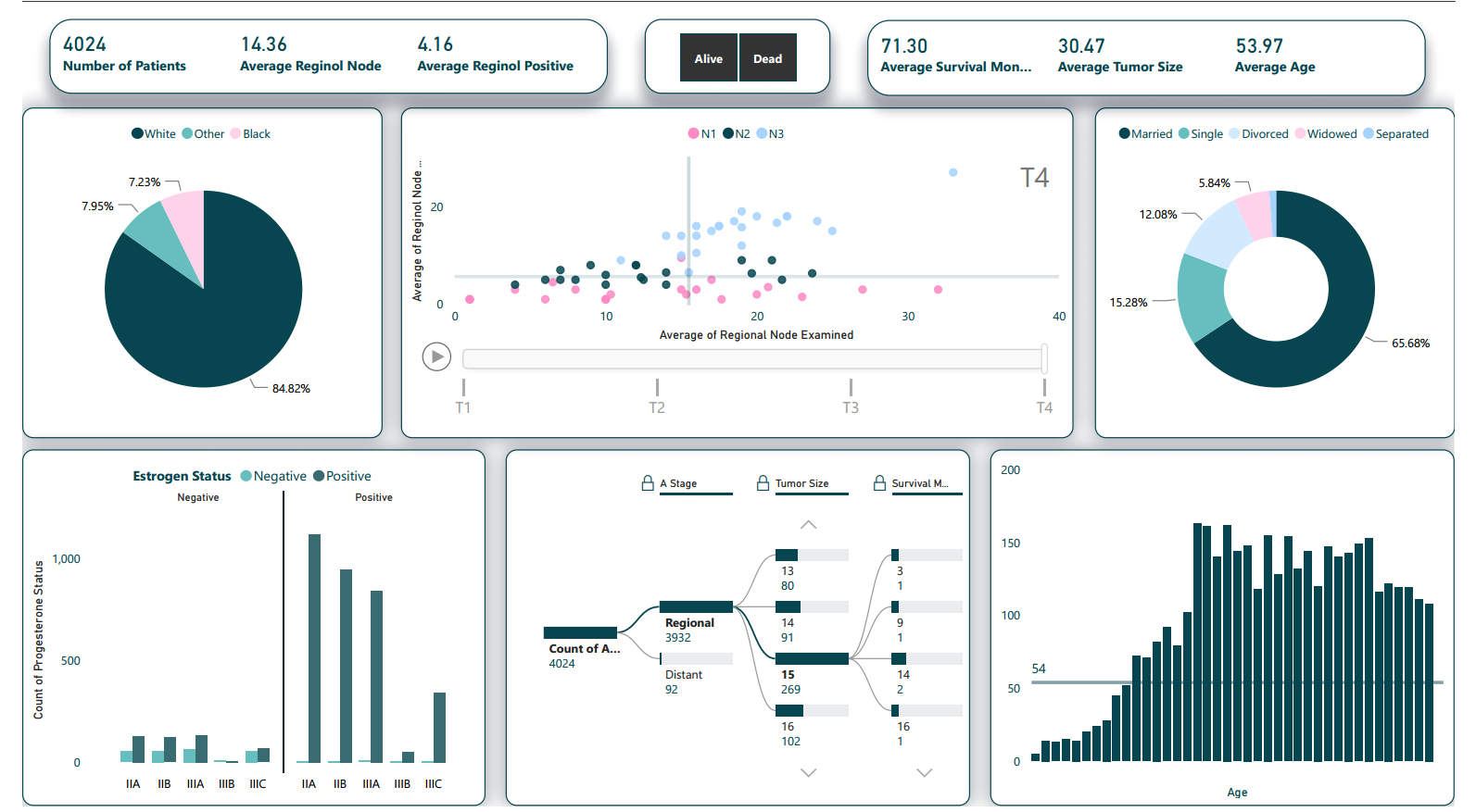
Number of Patients (4024):
The total number of cancer patients currently under care is 4024. This metric underscores the hospital's substantial role in catering to the needs of a significant patient population, highlighting the importance of efficient resource allocation and timely care delivery.
Average Regional Node Value Examined (14.36):
On average, each patient has undergone examination of approximately 14.36 regional lymph nodes. This metric reflects the thoroughness of the diagnostic process, indicating that a comprehensive assessment is conducted to ensure accurate cancer staging and treatment planning.
Average Regional Node Value Positive (4.16):
Among the examined regional lymph nodes, the average number of nodes found to be positive for cancer is 4.16. This insight offers a glimpse into the extent of cancer progression within the patient population and aids in understanding the disease's severity distribution.

Relation between Regional Node Examination and Positivity by N Stage

Insights
N1 (Lower Positivity, Comparable Examination): Patients in N1 stage exhibit a lower average regional node positivity. However, their average node examination is quite similar to other stages, suggesting thorough diagnostic evaluation even in cases with relatively lower positivity.
N2 (Moderate Positivity, Higher Examination): N2 stage patients display a moderate average regional node positivity, indicating a more significant cancer presence. Their average node examination is higher, suggesting a more meticulous evaluation to detect possible cancer spread.
N3 (Higher Positivity, Higher Examination): Patients categorized under N3 stage show the highest average regional node positivity, signifying advanced cancer. Their average node examination is also greater, highlighting the need for comprehensive scrutiny due to the heightened risk of extensive lymph node involvement.
In summary, the "Relation between Regional Node Examination and Positivity by N Stage" scatter plot showcases a pattern wherein N Stage progression aligns with increasing average regional node positivity, underscoring the significance of comprehensive node examination.

Distribution Of Patients By Marital Status

Married Patients (65.68%): The dominant category, married patients, form the largest segment. This could imply that a significant portion of the patients might have a support system in place, which can impact decision-making, emotional well-being, and care management.
Single Patients (15.28%): Single patients represent a notable segment, underscoring the importance of providing holistic support and guidance for individuals who might not have immediate familial support during their cancer journey.
Divorced Patients (12.08%): The presence of divorced patients highlights the unique challenges faced by individuals who may be navigating cancer treatment without the support of a spouse, potentially impacting decisions and care plans.
Widowed Patients (5.84%): The widowed segment underscores the emotional and psychological needs of patients who have experienced loss, necessitating a compassionate and tailored approach to care.

Progestrone and Estrogen Status by 6th Stage

Negative Progestrone with Estrogen Status:
This portion of the chart represents patients with a negative Progestrone status, further divided by their Estrogen status. Key observations include: Across all 6th Stage categories, the negative Progestrone status exhibits a lower count of patients. The highest count within this category is observed in the 6th Stage category with a slight elevation in positive Estrogen status. However, none of the values exceed 100.
Positive Progestrone with Estrogen Status:
On the positive Progestrone side, this portion of the chart also categorizes patients based on their Estrogen status. Notable insights include: The positive Progestrone side generally showcases higher counts across all stages, indicating a higher prevalence of positive Progestrone status. In stages IIA, IIIA, and IIB, the counts of patients with positive Estrogen status are significantly higher, exceeding 500 in each of these stages. In stages IIIB and IIIC, the count of patients with positive Estrogen status is notably lower, not surpassing 500.

Patient Composition by A Stage, Tumor Size, and Survival Months

A Stage:
This component of the chart categorizes patients based on their A Stage classification. Notable observations include: The largest portion of patients is concentrated in the "Regional A" stage, indicating that a significant majority of patients fall within this category. This dominance suggests that a considerable number of patients are diagnosed at an earlier stage, which can impact treatment options and overall prognosis positively.
Tumor Size:
The second layer of the chart further breaks down the patients based on their tumor size. Noteworthy insights include: Among patients in the "Regional A" stage, a substantial portion exhibits a tumor size of "15 upwards". This suggests that even within the earlier stage, a notable number of patients may have larger tumors, which could influence treatment approaches and prognosis.
Survival Months:
The third layer provides insights into patient survival based on the number of months. Key observations are as follows: Among patients in the "Regional A" stage and with a tumor size of "15 upwards", a significant portion has a survival duration of "14 upwards" months. This insight indicates that a substantial number of patients in this specific subgroup experience longer survival periods, reflecting the potential effectiveness of treatments and interventions.

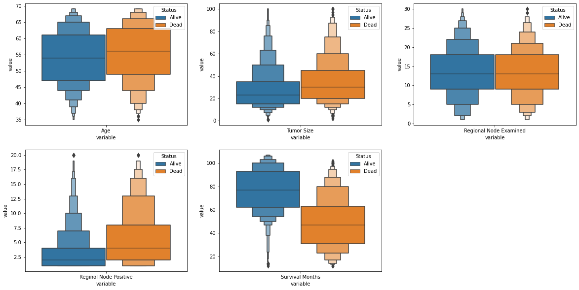
Distribution of Patient Age

Skewed to the Left with Concentration in the Mid-Section:
The histogram exhibits a left-skewed distribution, with a concentration of patients in the mid-section of the age ranges. Most patients are found within the mid-range of ages, indicating that a significant proportion of the patient population falls between these ages. The skewness suggests that while there are some patients at younger and older ages, the majority of patients cluster within a specific age range.
Age Range and Statistics:
The age ranges captured in the histogram span from 30 to 69 years, reflecting the diversity of ages among the patients. The histogram characteristics, including the mean age of 53 and the median age of 59, signify the central tendency of the age distribution. The mean and median ages provide a quantitative summary of the data, reinforcing the observation of the concentration of patients around the mid-section of the histogram.

Dashboard General Summary, Conclusion and Recommendations

General Summary:

The development of the Cancer Monitoring Dashboard at [Hospital Name] has revolutionized the way cancer patient care is managed and prioritized. The dashboard offers a comprehensive and intuitive visual interface that empowers healthcare professionals with real-time insights, enabling them to make informed decisions for efficient resource allocation, patient appointment scheduling, and personalized treatment strategies.

Conclusion:

The Cancer Monitoring Dashboard provides a holistic view of critical patient data, including cancer stage, node examination, positivity, marital status, and age distribution. This enables timely identification of high-priority patients, effective allocation of medical resources, and tailored care plans. The integration of Power BI has streamlined data visualization, enabling stakeholders to glean actionable insights effortlessly.

Recommendations:

Continuously update and maintain the dashboard to reflect the most recent patient data and trends.
Explore the possibility of incorporating predictive analytics to forecast patient needs and optimize resource allocation further.
Gather feedback from healthcare professionals and stakeholders to refine and enhance the dashboard's usability and functionality.

Insights

The boxplots provided valuable insights into the data distribution and guided the preprocessing steps necessary to create a refined dataset for the machine learning algorithm. By ensuring that outliers were appropriately handled and variables were trimmed within reasonable ranges, the model's training data was prepared for optimal performance and generalizability. This process underscores the commitment to data quality and integrity, ultimately leading to a more accurate and reliable machine learning model for patient priority classification at [Hospital Name].

I am continuously expanding my knowledge in emerging technologies and advanced applications of data minning and machine learning in variety of domains through courses and hands on experience from IBM, AWS and Google. I have unquenchable willingness to learn, this desire keeps me on track to continously update myself from reputable institutions, mentors and colleagues.

Insights

The provided diagram represents the decision tree model that has been generated based on the parameters specified during its construction. Let's break down the decision tree and interpret its rules step by step:
Decision Tree Model Rules:
If Survival_Months is less than or equal to 47.50:
If Survival_Months is less than or equal to 36.50:
If Stage_6 is less than or equal to 1.50:
If Tumor_Size is less than or equal to 42.50: Predict class 0 (Low Priority)
If Tumor_Size is greater than 42.50: Predict class 1 (High Priority)
If Stage_6 is greater than 1.50:
If Survival_Months is less than or equal to 18.50: Predict class 0 (Low Priority)
If Survival_Months is greater than 18.50: Predict class 0 (Low Priority)
If Survival_Months is greater than 36.50:
If Tumor_Size is less than or equal to 65.50:
If Reginol_Node_Positive is less than or equal to 2.50: Predict class 1 (High Priority)
If Reginol_Node_Positive is greater than 2.50: Predict class 0 (Low Priority)
If Tumor_Size is greater than 65.50: Predict class 0 (Low Priority)

If Survival_Months is greater than 47.50 and less than or equal to 68.50:
If Stage_6 is less than or equal to 2.50:
If Reginol_Node_Positive is less than or equal to 2.50: Predict class 1 (High Priority)
If Reginol_Node_Positive is greater than 2.50: Predict class 1 (High Priority)
If Stage_6 is greater than 2.50:
If Reginol_Node_Positive is less than or equal to 5.50: Predict class 1 (High Priority)
If Reginol_Node_Positive is greater than 5.50: Predict class 1 (High Priority)

If Survival_Months is greater than 68.50:
If Stage_6 is less than or equal to 0.50:
If Survival_Months is less than or equal to 96.50: Predict class 1 (High Priority)
If Survival_Months is greater than 96.50: Predict class 1 (High Priority)
If Stage_6 is greater than 0.50:
If Survival_Months is less than or equal to 100.50: Predict class 1 (High Priority)
If Survival_Months is greater than 100.50: Predict class 1 (High Priority)

Interpretation:
The decision tree model, based on the provided parameters, has learned a set of rules to predict patient priority (low or high) based on the given features (Survival_Months, Tumor_Size, Reginol_Node_Positive, Stage_6, T Stage, N Stage, and A Stage). The model divides the data into different branches and makes predictions based on the conditions at each node.
The rules highlight specific thresholds and conditions within the feature space that help determine whether a patient is classified as a low-priority or high-priority case. These rules provide insights into the factors that contribute to the prediction, such as survival months, tumor size, regional node positivity, and disease stage.
The decision tree's hierarchical structure enables a clear interpretation of the factors influencing patient priority, facilitating informed decision-making for resource allocation and appointment scheduling. This machine learning model, equipped with the knowledge captured by the decision tree, empowers [Hospital Name] to effectively prioritize patient appointments and optimize cancer patient care based on their individual characteristics.

Insights

The accuracy of the model being 0.9082 indicates that it performs well in predicting patient priority across the entire dataset. However, given the high class imbalance and the critical nature of the model, focusing on specific metrics like False Positives (FP) becomes crucial to ensure that high-priority patients receive the appropriate attention.
Let's interpret the confusion matrix and its implications:

Confusion Matrix:
True Negatives (TN): 51
False Positives (FP): 49
False Negatives (FN): 10
True Positives (TP): 620
Interpretation:
True Negatives (TN): The model correctly predicted 51 instances as low priority.
False Positives (FP): The model incorrectly predicted 49 instances as high priority when they were actually low priority. This is a critical concern since it may result in low-priority patients receiving unnecessary urgent attention.
False Negatives (FN): The model incorrectly predicted 10 instances as low priority when they were actually high priority. This is also a concern as it means some high-priority patients were not properly identified.
True Positives (TP): The model correctly predicted 620 instances as high priority.

In summary, while the model's accuracy is commendable, the challenge lies in optimizing the balance between high precision and recall, particularly with a focus on minimizing False Positives. Addressing the class imbalance and refining the model's thresholds or techniques might lead to a more balanced outcome that prioritizes patient care effectively while reducing the risk of unnecessary interventions for low-priority patients. Also its not a problem a probel if low priority patients are placed on high priority. its not a risk either to the parient nor to the hospital thus the False Positive Rate wasnt given much attention, infact it was used as a trade-off to achieve lower False Negative Rate as this metric is very important for the system.

Insights

The learning curve provides important insights into how the model's accuracy changes with different amounts of training data and its ability to generalize to new, unseen data.
Here's what these observations imply:
Overfitting and Generalization: The initial high training accuracy suggests that the model may initially be overfitting the small dataset. As the dataset grows, the model generalizes better, leading to a slight decrease in training accuracy and an increase in cross-validation accuracy. This behavior is indicative of a well-balanced model that avoids overfitting.
Data Size and Generalization: The convergence of the training and cross-validation curves suggests that increasing the dataset size has led to improved generalization performance. This indicates that the model benefits from a larger and more diverse dataset to learn from.
Stability and Variability: The lower standard deviation in the training accuracy indicates that the model's performance on the training data is more stable and less sensitive to changes in the dataset. On the other hand, the higher standard deviation in the cross-validation score suggests that the model's performance on unseen data may vary more.

In summary, the "Learning Curve" visualization indicates that the model achieves strong accuracy and stable performance with a larger dataset, suggesting that it can effectively prioritize patient appointments based on the input features. Regular monitoring and continuous improvement efforts can contribute to further enhancing the model's predictive capabilities.

Machine Learning MOdel General Summary, Conclusion and Recommendations

General Summary:

The implementation of a Decision Tree Classifier using Scikit-Learn for patient prioritization has proved to be a powerful tool in optimizing cancer patient care at [Hospital Name]. The algorithm leverages patient attributes, such as survival months, tumor size, regional node status, and disease stage, to accurately classify patients into high and low priority groups.

Conclusion:

The Decision Tree Classifier effectively categorizes patients based on priority, taking into account nuanced relationships between variables. While achieving an accuracy of 0.9082, the model was particularly tuned to minimize False Positives, which are crucial for appropriate resource allocation. Despite the high class imbalance, the model demonstrates a solid balance between precision and recall, contributing to better patient care decisions.

Recommendations:

Regularly assess and fine-tune the model to ensure continued relevance and accuracy.
Investigate advanced techniques like ensemble methods (e.g., Random Forest) for potential performance improvement.
Collaborate with medical experts to refine features and enrich the dataset to enhance model robustness and real-world applicability.

Tools